

A reliable A/B test sample size starts with the decision you need to make, not an industry benchmark. A checkout test may need enough eligible shoppers to detect a small lift, while a product-page test may measure a larger change with fewer exposures.
The calculation depends on your baseline conversion rate, minimum detectable effect, confidence level, statistical power, and traffic allocation. You also need a clear denominator, because visitors, users, sessions, and conversions are different measures. Start with that foundation before opening a sample-size calculator.
What Determines A/B Test Sample Size?
Sample size is the number of observations required to compare a control with one or more variants. In a standard ecommerce A/B test, the result should state whether the figure is per variation or total across all variations.
A result of 7,000 users per variation means 14,000 users for a two-arm test. That distinction matters when estimating traffic and duration.
Count the right unit
A visitor usually means a unique browser or device during a defined period. A user is a distinct person or account identifier, although logged-out shoppers can appear as different users across devices.
A session is one visit. The same visitor may create several sessions, so session-level data can overstate the amount of independent evidence when returning shoppers receive repeated exposure.
A conversion is the event you want to measure, such as a completed order, checkout completion, lead submission, or subscription. It isn’t the sample itself. The sample is the number of eligible visitors, users, or sessions, while conversions form the numerator in the conversion rate.
Match the sample unit to the randomization unit. If your platform assigns each user to a variation, measure conversion per user. If it assigns sessions, use session-level measurement and understand the limitations of repeat visits. Never divide user conversions by session counts.
Teams planning a design experiment can also review this ecommerce A/B testing playbook before choosing the primary metric and guardrails.
Define the conversion event
Choose one primary conversion before launch. For most stores, that may be an order per eligible visitor or user. A checkout test might instead use completed purchases among shoppers who reached the payment step.
Keep the observation window fixed. For example, count whether a user places an order within seven days of entering the experiment. Mixing same-session purchases with delayed purchases can change the meaning of the result.
A strong primary metric should connect directly to the decision. Add guardrails such as revenue per user, refund rate, payment failures, or customer-support contacts when a conversion lift could hide a quality problem.
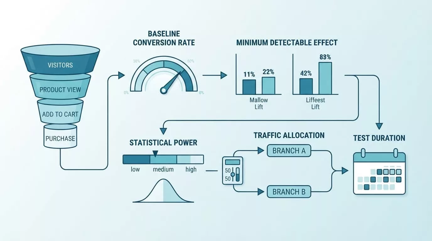
The Five Inputs Behind an A/B Test Sample Size
Most calculators ask for the same core assumptions. Each one changes the number of observations required, so avoid copying settings from a previous experiment without checking whether the business decision is the same.
Baseline conversion rate and detectable effect
The baseline conversion rate is the current performance of the control. Use recent, stable data for the exact audience, device mix, funnel step, and traffic source you plan to test.
The minimum detectable effect (MDE) is the smallest change that would justify action. Express it as an absolute difference or a relative lift. A move from 4% to 5% is a one-percentage-point absolute increase and a 25% relative lift.
Smaller effects require much larger samples. Because sample size is roughly proportional to the inverse square of the effect, cutting the MDE in half can require about four times as much traffic.
For a practical overview of these assumptions, see AB Tasty’s sample size calculation guidance.
Power and confidence level
Statistical power is the probability of detecting the chosen effect when it is real. Teams often use 80% power, while high-risk decisions may justify 90% or more.
A 95% confidence level commonly means a two-sided test with a 5% significance threshold. Raising confidence to 99% reduces the chance of a false positive, but it increases the required sample.
The usual starting point is 80% power and 95% confidence. Those settings aren’t universal rules. A low-risk button-color test and a major checkout rewrite may deserve different standards.
Statsig’s power analysis explanation describes how baseline rate, MDE, power, and significance work together.
Traffic allocation
A 50/50 split is usually the most efficient allocation for two variations because both groups reach the required sample at the same pace. An uneven split can make sense when the variant carries operational or financial risk, but it increases the total traffic needed.
The calculation also assumes two variations unless you specify otherwise. Adding more variants spreads traffic across more groups and increases the total sample required for reliable comparisons.
The same A/B test sample size per variation may stay unchanged with a different split, but the total number of visitors and the test duration will change.
How to Calculate A/B Test Sample Size
For a binary ecommerce metric, such as purchase or no purchase, use a two-proportion sample-size calculation. A normal-approximation formula for equal traffic allocation is:
n per variation ≈ [2p̄(1 – p̄)(z confidence + z power)²] / (p2 – p1)²
Here, p1 is the control conversion rate, p2 is the expected variant rate, and p̄ is their average. The z values come from your confidence and power settings.
Calculators may use exact methods, continuity corrections, or one-sided tests. Their results can differ slightly, so round up and keep the assumptions documented. Don’t treat a calculator’s output as valid if the input definitions don’t match your funnel.
Worked example with transparent assumptions
Suppose an online store tests a new checkout layout with these assumptions:
- The control converts 4% of eligible users.
- The team wants to detect an increase to 5%, an absolute MDE of 1 percentage point.
- The test uses 95% confidence and 80% power.
- Traffic is split 50/50 between control and variant.
- The primary metric is one completed order per eligible user.
Using the approximation, the average rate is 4.5%. The relevant z values are about 1.96 for confidence and 0.84 for power. The result is approximately 6,742 users per variation.
Round that figure to 7,000 users per variation, or 14,000 total eligible users for the two-arm experiment. The sample is users, not conversions. At a 4% control rate, those 14,000 users would produce roughly 560 control-equivalent conversions, but the calculation does not mean you should stop after reaching 560 orders.
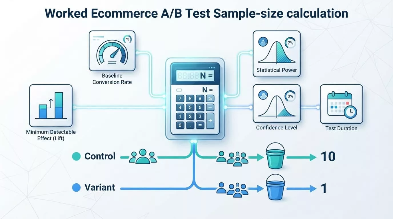
How changing the assumptions changes the result
| Changed assumption | Effect on required sample |
|---|---|
| A smaller MDE | Increases sample sharply, roughly with the square of the change |
| A lower baseline with the same relative lift | Often increases sample because the absolute difference becomes smaller |
| Higher statistical power | Increases sample and lowers the chance of missing a real effect |
| Higher confidence level | Increases sample and makes the significance threshold stricter |
| An uneven traffic split | Increases total traffic needed, even if the per-variation target stays similar |
Baseline changes need careful interpretation. If the rate falls from 4% to 2% while the relative MDE remains 25%, the target changes from 4% to 5% versus 2% to 2.5%. The latter has a smaller absolute difference, so it usually needs more users. If you hold the absolute one-point MDE constant instead, the result can move differently.
Turn Sample Size Into Test Duration
Once you know the required sample, divide it by the eligible traffic assigned to each variation. Use traffic that actually enters the experiment, not total site visits.
For the worked example, assume the store receives 20,000 eligible users per week. With a 50/50 split, each variation receives about 10,000 users weekly. The statistical target of 7,000 users per variation takes about 0.7 weeks.
That number is a planning estimate, not an automatic stopping date. Run the test through at least one complete business cycle. If weekday and weekend behavior differ, two full weekly cycles are safer than stopping after five high-traffic days. Monthly paydays, promotions, or replenishment patterns may require a longer window.
Account for traffic allocation
With a 60/40 split, the variant receives 40% of eligible traffic. To collect 7,000 variant users, the test needs at least 17,500 total users, compared with 14,000 at a 50/50 split.
A 90/10 split needs about 70,000 total users to provide 7,000 users in the smaller arm. The control reaches its target early, but the variant determines the schedule.
Use actual exposure rates when calculating duration. If only 70% of visitors load the tested checkout step, estimate time from that 70%, not from all homepage traffic.
Don’t stop because a dashboard turns green
Repeatedly checking results and stopping when significance appears can inflate false-positive risk. Set the sample target and minimum runtime before launch.
If traffic falls below forecast, extend the calendar rather than changing the MDE after seeing early results. A longer test is often better than a smaller, unstable test that misses the intended decision.
Validate the Experiment Before Trusting the Lift
A correct calculation can’t repair a broken experiment. Check implementation and audience quality before interpreting the conversion difference.
Investigate sample-ratio mismatch
A planned 50/50 allocation should produce close to a 50/50 observed split over time. Sample-ratio mismatch (SRM) occurs when the actual assignment differs beyond normal random variation, such as a persistent 55/45 result.
SRM can come from bucketing errors, redirects, targeting rules, consent handling, bot filters, or a tracking failure. Pause interpretation and inspect assignment logs, page exposure, browser behavior, and analytics filters before declaring a winner.
Also confirm that users remain in the same variation. If a returning shopper switches between control and variant, the groups no longer represent the planned comparison.
Watch novelty effects and overlapping tests
A new layout can change behavior because it feels unfamiliar. Early excitement or confusion may fade after shoppers return, so novelty effects are one reason to run across normal traffic cycles.
Overlapping experiments can create interaction effects. A checkout test and a shipping-message test may each look harmless alone but alter the same purchase decision when shown together. Separate audiences, coordinate launch dates, or design the assignment system to handle concurrent tests.
Review device type, browser, traffic source, customer status, and product category after the primary result. Segments can reveal a real usability issue, but avoid turning every segment into a separate winner claim.
An ecommerce analytics and testing checklist can help verify events such as add-to-cart, checkout start, payment failure, and completed order before launch.
Conclusion
The right A/B test sample size comes from the smallest business-relevant effect your funnel can detect with acceptable confidence and power. Define whether you are counting visitors, users, or sessions, then report every result as per variation or total.
For the example above, 7,000 users per variation is a planning target, not a universal ecommerce benchmark. Recalculate when the baseline rate, MDE, confidence level, power, traffic split, or audience changes, and keep the test running through a complete business cycle after the data pipeline passes its quality checks.